Ebola simulation part 1: early outbreak assessment
This practical simulates the early assessment and reconstruction of an Ebola Virus Disease (EVD) outbreak. It introduces various aspects of analysis of the early stage of an outbreak, including contact tracing data, epicurves, growth rate estimation from log-linear models, and more refined estimates of transmissibility. A follow-up practical will provide an introduction to transmission chain reconstruction using outbreaker2.
A novel EVD outbreak in Ankh, Republic of Morporkia
A new EVD outbreak has been notified in the small city of Ankh, located in the Northern, rural district of the Republic of Morporkia. Public Health Morporkia (PHM) is in charge of coordinating the outbreak response, and have contracted you as a consultant in epidemics analysis to inform the response in real time.
Required packages
The following packages are needed for this case study:
rioto read.xlsxfiles inggplot2for graphicsdplyrfor data handlingmagrittrfor data handlingoutbreaksfor some other outbreak datalinelistfor data cleaningincidencefor epidemic curves and basic model fittingepicontactsfor visualisation of contacts / transmission chainsdistcreteto obtain discretised delay distributionsepitrixto fit discretised Gamma distributionsearlyRto estimate R0projectionsfor short term forecasting of cases
For some of these packages, we recommend using the github (development) version, either because it is more up-to-date, or because they have not been released on CRAN yet.
We provide installation commands for each package; not that you only need to install these packages if they are not already present on your system.
## instructions for CRAN packages
install.packages("rio")
install.packages("ggplot2")
install.packages("dplyr")
install.packages("magrittr")
install.packages("outbreaks")
install.packages("incidence")
install.packages("distcrete")
install.packages("epitrix")
## instructions for github packages (latest versions)
remotes::install_github("reconhub/epicontacts")
remotes::install_github("reconhub/linelist")
remotes::install_github("reconhub/earlyR")
remotes::install_github("reconhub/projections")The RECON deployer should contain all the right versions of the different packages; if you are using a deployer, you can install all needed packages by:
go to the deployer, double-click on the
.Rprojfile to open a new Rstudio session in the right folder (no need to close the session you have opened for the practical)type the instructions below:
## activate the deployer
source("activate.R")
## install packages from the deployer
install.packages("rio")
install.packages("ggplot2")
install.packages("dplyr")
install.packages("magrittr")
install.packages("outbreaks")
install.packages("incidence")
install.packages("distcrete")
install.packages("epitrix")
install.packages("epicontacts")
install.packages("linelist")
install.packages("earlyR")
install.packages("projections")To load these packages, type:
library(rio)
library(ggplot2)
library(dplyr)
library(magrittr)
library(outbreaks)
library(incidence)
library(epicontacts)
library(linelist)
library(distcrete)
library(epitrix)
library(earlyR)
library(projections)Importing data
While a new data update is pending, you have been given the following linelist and contact data, from the early stages of the outbreak:
phm_evd_linelist_2017-10-27.xlsx: a linelist containing case information up to the 27th October 2017
phm_evd_contacts_2017-10-27.xlsx: a list of contacts reported between cases up to the 27th October 2017, where
fromindicates a potential source of infection, andtothe recipient of the contact.
To read into R, download these files and use the function read_xlsx() from the readxl package to import the data. Each import will create a data table stored as a tibble object. Call the first one linelist, and the second one contacts. For instance, you first command line could look like:
linelist <- rio::import("phm_evd_linelist-2017-10-27.xlsx")Note that for further analyses, you will need to make sure all dates are stored as Date objects. This could be done manually using as.Date, but will be taken care of here using linelist’s clean_data:
Data cleaning
Once imported, the raw data should look like:
## linelist: one line per case
linelist_raw
## id Date of Onset Date.Report. SEX. Âge location
## 1 39e9dc 43018 43030 Female 62 Pseudopolis
## 2 664549 43024 43032 Male 28 peudopolis
## 3 B4D8AA 43025 “23/10/2017” male 54 Ankh-Morpork
## 4 51883d “18// 10/2017” 22-10-2017 male 57 PSEUDOPOLIS
## 5 947e40 43028 “2017/10/25” f 23 Ankh Morpork
## 6 9aa197 43028 “2017-10-23” f 66 AM
## 7 e4b0a2 43029 “2017-10-24” female 13 Ankh Morpork
## 8 AF0AC0 “2017-10-21” “26-10-2017” M 10 ankh morpork
## 9 185911 “2017-10-21” “26-10-2017” female 34 AM
## 10 601D2E “2017/10/22” “28-10-2017” <NA> 11 AM
## 11 605322 43030 “28 / 10 / 2017” FEMALE 23 Ankh Morpork
## 12 E399B1 23 / 10 / 2017 “28/10/2017” female 23 Ankh Morpork
## contacts: pairs of cases with reported contacts
contacts_raw
## Source Case #ID case.id
## 1 51883d 185911
## 2 b4d8aa e4b0a2
## 3 39e9dc b4d8aa
## 4 39E9DC 601d2e
## 5 51883d 9AA197
## 6 39e9dc 51883d
## 7 39E9DC e399b1
## 8 b4d8aa AF0AC0
## 9 39E9DC 947e40
## 10 39E9DC 664549
## 11 39e9dc 605322Examine these data and try to list existing issues.
The raw data, whilst very small in size, have a number of issues, including:
capitalisation: mixture of upper case and lower cases
dates: their format is very heterogeneous, so that dates are not readily useable
special characters: accents, various separators and trailing / heading white spaces
typos / inconsistent coding: gender is sometimes indicated in full words, sometimes abbreviated; location has some obvious abbreviations and typos
We will use the function clean_data() from the linelist package to clean these data. This function will:
- set all characters to lower case
- use
_as universal separator - remove all heading and trailing separators
- replace all accentuated characters by their closest ASCII match
- detect date formats and convert entries to
Datewhen relevant (see argumentguess_dates) - replace typos and recode variables (see argument
wordlists)
For this last part, we need to load a separate file containing cleaning rules: phm_evd_cleaning_rules.xlsx.
Examine this file (and read the ‘explanations’ tab), import it as the other files, and save the resulting data.frame as and object called cleaning_rules. The output should look like:
cleaning_rules
## bad_spelling good_spelling variable
## 1 f female sex
## 2 m male sex
## 3 .missing unknown sex
## 4 am ankh_morpork location
## 5 peudopolis pseudopolis location
## 6 .missing unknown locationWe can now clean our data using clean_data; execute and interprete the following commands:
## clean linelist
linelist <- linelist_raw %>%
clean_data(wordlist = cleaning_rules) %>%
mutate_at(vars(contains("date")), guess_dates)
linelist
## id date_of_onset date_report sex age location
## 1 39e9dc 2017-10-10 2017-10-22 female 62 pseudopolis
## 2 664549 2017-10-16 2017-10-24 male 28 pseudopolis
## 3 b4d8aa 2017-10-17 2017-10-23 male 54 ankh_morpork
## 4 51883d 2017-10-18 2017-10-22 male 57 pseudopolis
## 5 947e40 2017-10-20 2017-10-25 female 23 ankh_morpork
## 6 9aa197 2017-10-20 2017-10-23 female 66 ankh_morpork
## 7 e4b0a2 2017-10-21 2017-10-24 female 13 ankh_morpork
## 8 af0ac0 2017-10-21 2017-10-26 male 10 ankh_morpork
## 9 185911 2017-10-21 2017-10-26 female 34 ankh_morpork
## 10 601d2e 2017-10-22 2017-10-28 unknown 11 ankh_morpork
## 11 605322 2017-10-22 2017-10-28 female 23 ankh_morpork
## 12 e399b1 2017-10-23 2017-10-28 female 23 ankh_morpork
## clean contacts
contacts <- clean_data(contacts_raw)
contacts
## source_case_id case_id
## 1 51883d 185911
## 2 b4d8aa e4b0a2
## 3 39e9dc b4d8aa
## 4 39e9dc 601d2e
## 5 51883d 9aa197
## 6 39e9dc 51883d
## 7 39e9dc e399b1
## 8 b4d8aa af0ac0
## 9 39e9dc 947e40
## 10 39e9dc 664549
## 11 39e9dc 605322Descriptive analyses
A first look at contacts
Contact tracing is at the centre of an Ebola outbreak response. Using the function make_epicontacts in the epicontacts package, create a new epicontacts object called x. The result should look like:
x
##
## /// Epidemiological Contacts //
##
## // class: epicontacts
## // 12 cases in linelist; 11 contacts; directed
##
## // linelist
##
## # A tibble: 12 x 6
## id date_of_onset date_report sex age location
## <chr> <date> <date> <chr> <dbl> <chr>
## 1 39e9dc 2017-10-10 2017-10-22 female 62 pseudopolis
## 2 664549 2017-10-16 2017-10-24 male 28 pseudopolis
## 3 b4d8aa 2017-10-17 2017-10-23 male 54 ankh_morpork
## 4 51883d 2017-10-18 2017-10-22 male 57 pseudopolis
## 5 947e40 2017-10-20 2017-10-25 female 23 ankh_morpork
## 6 9aa197 2017-10-20 2017-10-23 female 66 ankh_morpork
## 7 e4b0a2 2017-10-21 2017-10-24 female 13 ankh_morpork
## 8 af0ac0 2017-10-21 2017-10-26 male 10 ankh_morpork
## 9 185911 2017-10-21 2017-10-26 female 34 ankh_morpork
## 10 601d2e 2017-10-22 2017-10-28 unknown 11 ankh_morpork
## 11 605322 2017-10-22 2017-10-28 female 23 ankh_morpork
## 12 e399b1 2017-10-23 2017-10-28 female 23 ankh_morpork
##
## // contacts
##
## # A tibble: 11 x 2
## from to
## <chr> <chr>
## 1 51883d 185911
## 2 b4d8aa e4b0a2
## 3 39e9dc b4d8aa
## 4 39e9dc 601d2e
## 5 51883d 9aa197
## 6 39e9dc 51883d
## 7 39e9dc e399b1
## 8 b4d8aa af0ac0
## 9 39e9dc 947e40
## 10 39e9dc 664549
## 11 39e9dc 605322You can easily plot these contacts, but with a little bit of tweaking (see ?vis_epicontacts) you can customise shapes by gender:
p <- plot(x, node_shape = "sex",
shapes = c(male = "male", female = "female", unknown = "question-circle"),
selector = FALSE)
## pWhat can you say about these contacts?
Looking at incidence curves
The first question PHM asks you is simply: how bad is it?. Given that this is a terrible disease, with a mortality rate nearing 70%, there is a lot of concern about this outbreak getting out of control. The first step of the analysis lies in drawing an epicurve, i.e. an plot of incidence over time.
Using the package incidence, compute daily incidence based on the dates of symptom onset. Store the result in an object called i; the result should look like (pending some fine tweaking, which you should feel free to ignore if this is your first time using ggplot2):
i
## <incidence object>
## [12 cases from days 2017-10-10 to 2017-10-23]
##
## $counts: matrix with 14 rows and 1 columns
## $n: 12 cases in total
## $dates: 14 dates marking the left-side of bins
## $interval: 1 day
## $timespan: 14 days
## $cumulative: FALSE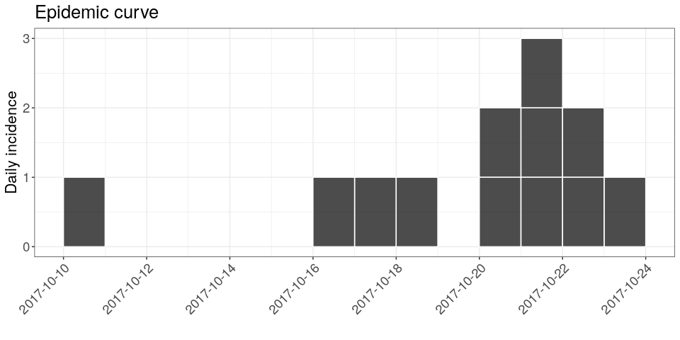
we provide two items large_txt and rotate_x_txt which you can add to your ggplot object to mimic the graph above:
large_txt <- ggplot2::theme(text = ggplot2::element_text(size = 16),
axis.text = ggplot2::element_text(size = 12))
rotate_x_txt <- theme(axis.text.x = element_text(angle = 45,
hjust = 1))If you pay close attention to the dates on the x-axis, you may notice that something is missing. Indeed, the graph stops right after the last case, while the data should be complete until the 27th October 2017. You can remedy this using the argument last_date in the incidence function:
database_date <- as.Date("2017-10-27")
i <- incidence(linelist$date_of_onset, last_date = database_date)
i
## <incidence object>
## [12 cases from days 2017-10-10 to 2017-10-27]
##
## $counts: matrix with 18 rows and 1 columns
## $n: 12 cases in total
## $dates: 18 dates marking the left-side of bins
## $interval: 1 day
## $timespan: 18 days
## $cumulative: FALSE
plot(i, show_cases = TRUE) +
theme_bw() +
large_txt +
rotate_x_txt +
labs(title = sprintf("Epidemic curve as of the %s", database_date))
Statistical analyses
Log-linear model
The simplest model of incidence is probably the log-linear model, i.e. a linear regression on log-transformed incidences. In the incidence package, the function fit will estimate the parameters of this model from an incidence object (here, i). Apply it to the data and store the result in a new object called f. You can print f to derive estimates of the growth rate r and the doubling time, and add the corresponding model to the incidence plot:
f <- fit(i)
## Warning in fit(i): 10 dates with incidence of 0 ignored for fitting
f
## <incidence_fit object>
##
## $model: regression of log-incidence over time
##
## $info: list containing the following items:
## $r (daily growth rate):
## [1] 0.05352107
##
## $r.conf (confidence interval):
## 2.5 % 97.5 %
## [1,] -0.0390633 0.1461054
##
## $doubling (doubling time in days):
## [1] 12.95092
##
## $doubling.conf (confidence interval):
## 2.5 % 97.5 %
## [1,] 4.744158 -17.74421
##
## $pred: data.frame of incidence predictions (8 rows, 5 columns)
plot(i, show_cases = TRUE, fit = f) +
theme_bw() +
large_txt +
rotate_x_txt +
labs(title = "Epidemic curve and log-linear fit")
## the argument `show_cases` requires the argument `stack = TRUE`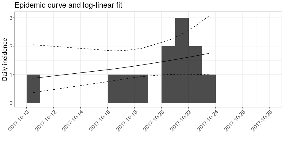
How would you interpret this result?What criticism would you make on this model?
Estimation of transmissibility (R)
Branching process model
The transmissibility of the disease can be assessed through the estimation of the reproduction number R, defined as the number of expected secondary cases per infected case. In the early stages of an outbreak, and assuming no immunity in the population, this quantity is also the basic reproduction number R0, i.e. R in a fully susceptible population.
The package earlyR implements a simple maximum-likelihood estimation of R, using dates of onset of symptoms and information on the serial interval distribution. It is a simpler but less flexible version of the model by Cori et al (2013, AJE 178: 1505–1512) implemented in EpiEstim.
Briefly, earlyR uses a simple model describing incidence on a given day as a Poisson process determined by a global force of infection on that day:
xt ∼ 𝒫(λt)
where xt is the incidence (based on symptom onset) on day t and λt is the force of infection. Noting R the reproduction number and w() the discrete serial interval distribution, we have:
$$ \lambda_t = R * \sum_{s=1}^t x_s w(t - s) $$
The likelihood (probability of observing the data given the model and parameters) is defined as a function of R:
$$ \mathcal{L}(x) = p(x | R) = \prod_{t=1}^T F_{\mathcal{P}}(x_t, \lambda_t) $$
where F𝒫 is the Poisson probability mass function.
Looking into the past: estimating the serial interval from older data
As current data are insufficient to estimate the serial interval distribution, some colleague recommends using data from a past outbreak stored in the outbreaks package, as the dataset ebola_sim_clean. Load this dataset, and create a new epicontacts object as before, without plotting it (it is a much larger dataset). Store the new object as old_evd; the output should look like:
old_evd
##
## /// Epidemiological Contacts //
##
## // class: epicontacts
## // 5,829 cases in linelist; 3,800 contacts; directed
##
## // linelist
##
## # A tibble: 5,829 x 11
## id generation date_of_infecti… date_of_onset date_of_hospita…
## <chr> <int> <date> <date> <date>
## 1 d1fa… 0 NA 2014-04-07 2014-04-17
## 2 5337… 1 2014-04-09 2014-04-15 2014-04-20
## 3 f5c3… 1 2014-04-18 2014-04-21 2014-04-25
## 4 6c28… 2 NA 2014-04-27 2014-04-27
## 5 0f58… 2 2014-04-22 2014-04-26 2014-04-29
## 6 4973… 0 2014-03-19 2014-04-25 2014-05-02
## 7 f914… 3 NA 2014-05-03 2014-05-04
## 8 881b… 3 2014-04-26 2014-05-01 2014-05-05
## 9 e66f… 2 NA 2014-04-21 2014-05-06
## 10 20b6… 3 NA 2014-05-05 2014-05-06
## # … with 5,819 more rows, and 6 more variables: date_of_outcome <date>,
## # outcome <fct>, gender <fct>, hospital <fct>, lon <dbl>, lat <dbl>
##
## // contacts
##
## # A tibble: 3,800 x 3
## from to source
## <chr> <chr> <fct>
## 1 d1fafd 53371b other
## 2 cac51e f5c3d8 funeral
## 3 f5c3d8 0f58c4 other
## 4 0f58c4 881bd4 other
## 5 8508df 40ae5f other
## 6 127d83 f547d6 funeral
## 7 f5c3d8 d58402 other
## 8 20b688 d8a13d other
## 9 2ae019 a3c8b8 other
## 10 20b688 974bc1 other
## # … with 3,790 more rowsThe function get_pairwise can be used to extract pairwise features of contacts based on attributes of the linelist. For instance, it could be used to test for assortativity, but also to compute delays between connected cases. Here, we use it to extract the serial interval:
old_si <- get_pairwise(old_evd, "date_of_onset")
summary(old_si)
## Min. 1st Qu. Median Mean 3rd Qu. Max. NA's
## 1.00 5.00 9.00 11.06 15.00 99.00 1684
old_si <- na.omit(old_si)
summary(old_si)
## Min. 1st Qu. Median Mean 3rd Qu. Max.
## 1.00 5.00 9.00 11.06 15.00 99.00
hist(old_si, xlab = "Days after symptom onset", ylab = "Frequency",
main = "Serial interval (empirical distribution)",
col = "grey", border = "white")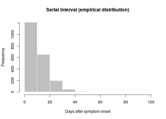
What do you think of this distribution? Make the adjustments you deem necessary, and then use the function fit_disc_gamma from the package epitrix to fit a discretised Gamma distribution to these data. Your results should approximately look like:
si_fit <- fit_disc_gamma(old_si)
si_fit
## $mu
## [1] 11.48373
##
## $cv
## [1] 0.6429561
##
## $sd
## [1] 7.383534
##
## $ll
## [1] -6905.588
##
## $converged
## [1] TRUE
##
## $distribution
## A discrete distribution
## name: gamma
## parameters:
## shape: 2.41900859135364
## scale: 4.74728799288241si_fit contains various information about the fitted delays, including the estimated distribution in the $distribution slot. You can compare this distribution to the empirical data in the following plot:
si <- si_fit$distribution
si
## A discrete distribution
## name: gamma
## parameters:
## shape: 2.41900859135364
## scale: 4.74728799288241
## compare fitted distribution to data
hist(old_si, xlab = "Days after symptom onset", ylab = "Frequency",
main = "Serial interval: fit to data", col = "salmon", border = "white",
nclass = 50, ylim = c(0, 0.07), prob = TRUE)
points(0:60, si$d(0:60), col = "#9933ff", pch = 20)
points(0:60, si$d(0:60), col = "#9933ff", type = "l", lty = 2)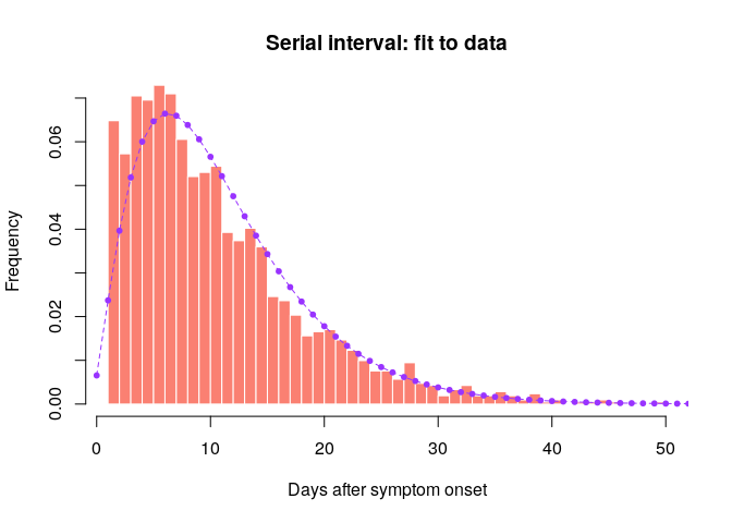
Would you trust this estimation of the generation time? How would you compare it to actual estimates from the West African EVD outbreak (WHO Ebola Response Team (2014) NEJM 371:1481–1495) with a mean of 15.3 days and a standard deviation 9.3 days?
Back to the future: estimation of R0 in the current outbreak
Now that we have estimates of the serial interval based on a previous outbreak, we can use this information to estimate transmissibility of the disease (as measured by R0) in the current outbreak.
Using the estimates of the mean and standard deviation of the serial interval you just obtained, use the function get_R to estimate the reproduction number, specifying a maximum R of 10 (see ?get_R) and store the result in a new object R:
You can visualise the results as follows:
R
##
## /// Early estimate of reproduction number (R) //
## // class: earlyR, list
##
## // Maximum-Likelihood estimate of R ($R_ml):
## [1] 2.042042
##
##
## // $lambda:
## NA 0.04088711 0.05343783 0.06188455 0.06668495 0.06850099...
##
## // $dates:
## [1] "2017-10-10" "2017-10-11" "2017-10-12" "2017-10-13" "2017-10-14"
## [6] "2017-10-15"
## ...
##
## // $si (serial interval):
## A discrete distribution
## name: gamma
## parameters:
## shape: 2.41900859135364
## scale: 4.74728799288241
plot(R) +
geom_vline(xintercept = 1, color = "#ac3973") +
theme_bw() +
large_txt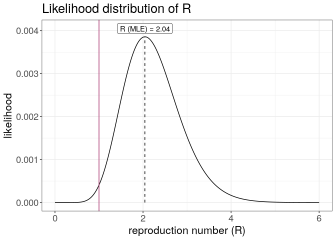
plot(R, "lambdas") +
theme_bw() +
large_txt
## Warning: Removed 1 rows containing missing values (position_stack).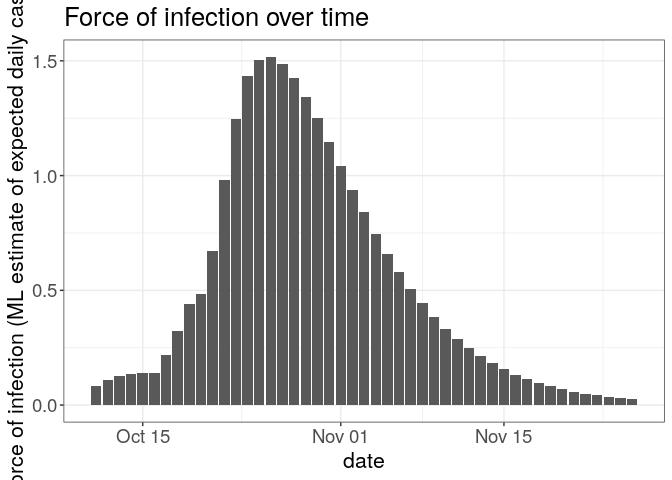
The first figure shows the distribution of likely values of R, and the Maximum-Likelihood (ML) estimation. The second figure shows the global force of infection over time, with dashed bars indicating dates of onset of the cases.
Interpret these results: what do you make of the reproduction number?What does it reflect? Based on the last part of the epicurve, some colleagues suggest that incidence is going down and the outbreak may be under control. What is your opinion on this?
Short-term forecasting
The function project from the package projections can be used to simulate plausible epidemic trajectories by simulating daily incidence using the same branching process as the one used to estimate R0 in earlyR. All that is needed is one or several values of R0 and a serial interval distribution, stored as a distcrete object.
Here, we illustrate how we can simulate 5 random trajectories using a fixed value of R0 = 2.04, the ML estimate of R0:
library(projections)
project(i, R = R$R_ml, si = si, n_sim = 5, n_days = 10, R_fix_within = TRUE)
##
## /// Incidence projections //
##
## // class: projections, matrix
## // 10 dates (rows); 5 simulations (columns)
##
## // first rows/columns:
## [,1] [,2] [,3] [,4] [,5]
## 2017-10-28 1 1 0 1 0
## 2017-10-29 1 3 1 5 0
## 2017-10-30 1 0 6 0 0
## 2017-10-31 2 1 1 0 0
## .
## .
## .
##
## // dates:
## [1] "2017-10-28" "2017-10-29" "2017-10-30" "2017-10-31" "2017-11-01"
## [6] "2017-11-02" "2017-11-03" "2017-11-04" "2017-11-05" "2017-11-06"Using the same principle, generate 1,000 trajectories for the next 2 weeks, using a range of plausible values of R0. Note that you can use sample_R to obtain these values from your earlyR object. Store your results in an object called proj. Plotting the results should give something akin to:
plot(i) %>%
add_projections(proj, c(.1, .5, .9)) +
theme_bw() +
scale_x_date() +
large_txt +
rotate_x_txt +
labs(title = "Short term forcasting of new cases")
## Scale for 'x' is already present. Adding another scale for 'x', which
## will replace the existing scale.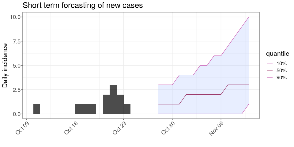
Interpret the following summary:
apply(proj, 1, summary)
## 2017-10-28 2017-10-29 2017-10-30 2017-10-31 2017-11-01 2017-11-02
## Min. 0.000 0.000 0.000 0.000 0.000 0.000
## 1st Qu. 1.000 0.750 1.000 1.000 1.000 1.000
## Median 1.000 1.000 1.000 1.000 2.000 2.000
## Mean 1.584 1.541 1.693 1.796 1.884 2.073
## 3rd Qu. 2.000 2.000 2.000 3.000 3.000 3.000
## Max. 8.000 9.000 8.000 8.000 10.000 9.000
## 2017-11-03 2017-11-04 2017-11-05 2017-11-06 2017-11-07 2017-11-08
## Min. 0.000 0.000 0.000 0.000 0.000 0.000
## 1st Qu. 1.000 1.000 1.000 1.000 1.000 1.000
## Median 2.000 2.000 2.000 2.000 3.000 3.000
## Mean 2.356 2.469 2.715 3.104 3.402 3.869
## 3rd Qu. 3.000 3.000 4.000 4.000 5.000 5.000
## Max. 10.000 16.000 19.000 20.000 24.000 34.000
## 2017-11-09 2017-11-10
## Min. 0.000 0.000
## 1st Qu. 1.000 2.000
## Median 3.000 3.000
## Mean 4.265 4.834
## 3rd Qu. 6.000 6.000
## Max. 33.000 40.000
apply(proj, 1, function(x) mean(x>0))
## 2017-10-28 2017-10-29 2017-10-30 2017-10-31 2017-11-01 2017-11-02
## 0.787 0.750 0.802 0.790 0.795 0.810
## 2017-11-03 2017-11-04 2017-11-05 2017-11-06 2017-11-07 2017-11-08
## 0.853 0.840 0.847 0.881 0.885 0.896
## 2017-11-09 2017-11-10
## 0.892 0.926According to these results, what are the chances that more cases will appear in the near future?Is this outbreak being brought under control? Would you recommend scaling up / down the response?
Follow-up…
For a follow-up on this outbreak, have a look at the second part of this simulated response, which includes a data update, genetic sequences, and the use of outbreak reconstruction tools.
About this document
Contributors
- Thibaut Jombart: initial version
Contributions are welcome via pull requests. The source file is hosted on github.
Legal stuff
License: CC-BY Copyright: Thibaut Jombart, 2017
