TB: exploring the case of TB elimination with a simple compartmental model

13 June 2019 / [practicals] / #tuberculosis

Eliminating tuberculosis (TB) is now a priority in the Global Health agenda. Is it achievable? How and when could this happen? Though still uncertain, it is an ongoing discussion in the field. In this practical, we will illustrate important concepts of TB epidemiology with a simple compartmental model and assess the interventions required to achieve elimination thresholds and End TB goals set by the World Health Organization (WHO).

Core concepts

The following concepts will be developed during the practical:

Compartmental models
Flow diagrams
Long-term infection dynamics
Natural history of TB
TB control strategies

Required packages

# install.packages("deSolve", dep = TRUE)
# install.packages("gridExtra", dep = TRUE)
# install.packages("ggplot2", dep = TRUE)

Part I: Set up a basic TB model

Natural History of TB

Tuberculosis is an infectious disease caused by Mycobacterium tuberculosis. Pulmonary tuberculosis (PTB) is the most common manifestation of the disease and the form most likely to be infectious. TB is transmitted from person to person through the air. Studies of household contacts and phylogenetic analyses have estimated the transmission potential of the average infectious TB case to be between 4 and 18 secondary cases per year (1).

An important feature of TB infection is the latent period. The vast majority of newly infected individuals progress to a latent stage in which M. tuberculosis remains dormant and does not replicate. People in this stage are non-infectious. Many people with latent TB will never progress to active disease. At the population level, approximately 10% of latent infections will break out into active disease over a lifetime (2). We also know that about 10% of new TB transmission events will fast-track to active TB disease (3). Active TB cases are symptomatic and infectious. Although intermediate stages of subclinical active TB are currently recognized, for simplicity we will assume symptomatic disease cases are infectious.

The average duration of the infectious period is about 3 years. Cohort studies have established that after this period, roughly 50% of active TB cases die from the disease, while the other 50% recover spontaneously (4). TB does not confer complete immunity after recovery; however, partial immunity has been observed in previously infected individuals and might protect from reinfection (hazard ratio ~0.5) (5). Finally, individuals who recover from active TB are not only susceptible to re-infection, but they can also relapse into active disease, usually at a yearly rate of around 0.5% (6).

1) Following the statement above, can you complete the table of parameters? Draw a flow chart if necessary.

(Note: All parameters with prefix T. are in a scale of time (years). Use these parameters to calculate the missing rates as necessary).

First, let’s load some libraries.

# Load packages
library(deSolve)
library(gridExtra)
library(ggplot2)
library(reshape)

Now, complete the parameter list below:

# Model Parameters
T.lfx    <- 72              # Life expectancy
T.dur    <-                 # Duration of infectious period
beta     <-                 # Transmission rate per capita
break_in <-                 # Transition rate from latent to active disease
selfcure <-                 # Rate of spontaneous cure
mu       <- 1/T.lfx         # Background mortality rate
mu_tb    <-                 # TB mortality rate
fast     <-                 # Fraction fast progressing to active TB
imm      <-                 # Infectiousness decline (partial immunity)
relapse  <-                 # Relapse rate

The code below describes the set of ordinary differential equations that describe the system. Each equation (named with prefix d) represents a compartment in the model with respective flows in and out, at each time step.

In order to track epidemic changes over time and under different interventions, we need to code model outputs for the recent and remote incidence components.

2) Look at the code below. Using the rates and stages in the first equations, code the model outputs for remote and recent TB incidence:

Copy and paste the code below

TB.Basic <- function (t, state, parameters) {
  with(as.list(c(state, parameters)),             
       {
         N      <- U + L + I + R            # Total population
         births <- I * mu_tb + N * mu       # Births (for stable population)
         lambda <- beta * I/N               # Force of Infection
         
         # Uninfected 
         dU <- births - U * (lambda + mu)                              
         
         # Latent 
         dL <- U * lambda * (1-fast) + R * (lambda * (1-fast) * imm) - L * (mu + break_in) 
         
         # Active TB
         dI <- U * lambda * fast + R * (lambda * fast * imm) +  L * break_in + R * relapse -
               I * (mu + mu_tb + selfcure)
         
         # Recovered
         dR <- I * selfcure - R * (lambda * imm + relapse + mu)      
         
         # Model outcomes
         dIncidence <- U * (lambda * fast) + R * (lambda * fast * imm) + L * break_in + R * relapse 
         
         # ::::::::: TRY  TO COMPLETE THIS EQUATIONS 
         
         dIrecent   <-

         dIremote   <-
        
         # ::::::::::::::::::::::::::::::::::::::::::::
           
         # wrap-up 
         dx <- c(dU, dL, dI, dR, dIncidence, dIrecent, dIremote)
         list(dx)
       }
  )
}

3) Looking at the code above, can you write down (on paper) the differential equations for this model?

Now that the model is coded and parameterised, let’s run the code and evaluate TB incidence.

Note: in the code below, we create a handy function that will help us run the models under different conditions and returns some plots and data. We will call this function (get_intervention) repeatedly during the practical.

(Note: for this section, copy and paste the code shown and try to understand what is going on in each section. Hopefully, commenting in the code is transparent enough! Organise your own script in sections to keep track of the exercise)

Copy and paste the code below

get_intervention <- function(sfin, params_new, params_old, times_new,
                             t.interv, fx_scale, fx_basic, int_name, data_stub) {

  # Starting conditions
  xstart <- c(U = sfin$U,
              L = sfin$L,
              I = sfin$I,
              R = sfin$R,
              Incidence = sfin$Incidence,
              Irecent   = sfin$Irecent,
              Iremote   = sfin$Iremote)

  # Select type of function
  if (is.na(t.interv)) {
    fx <- fx_basic
  }  else {
    fx <- fx_scale
  }
  
  # Run the model
  out <- as.data.frame(ode(y = xstart, times = times_new,
                           func = fx, parms = params_new)) 
  # Model output
  N           <- out$U + out$L + out$I + out$R
  rate.inc    <- 1e5 * (diff(out$Incidence) / N[1:length(N) - 1])
  fr.remo     <- diff(out$Iremote) / diff(out$Incidence)
  time        <- out$time[1:length(out$time) - 1]
  dat         <- data.frame(Years = time + (2019 - 400), Incidence = rate.inc)
  dat$Sim     <- int_name

  # If it is a first run, nothing to append 
  if (is.na(data_stub)) {
    data <- dat
  }
  else # Append previous runs
  {
    data <- rbind(data_stub, dat)
  }

  remote <- fr.remo  # rename a variable with the fraction of remote incidence
  titl   <- int_name

  p <- ggplot(data = data, mapping = aes(x = Years, y = Incidence, col = Sim))
  p1 <- p +
    geom_line(size = 1.2) +
    ggtitle ("TB Incidence") +
    theme_bw() + ylab("Rate per 100, 000 pop") +
    ylim(0, max(data$Incidence))

  df <- data.frame(
    Source = c("Recent", "Remote"),
    value  = c(1 - tail(remote, 1), tail(remote, 1))
  )

  # Pie chart of remote vs recent incidence 
  mycols <- c("#0073C2FF", "#EFC000FF")
  pie <- ggplot(df, aes(x = "", y = value, fill = Source)) +
    geom_bar(width = 1, stat = "identity") +
    coord_polar("y", start = 0) +
    scale_fill_manual(values = mycols) +
    theme_void() +
    ggtitle(titl)

  output <- list("out" = out, "lines" = p1, "pie" = pie, "data" = data)

  # Return the results
  return(output)
}

Set some simulation parameters

Copy and paste the code below

t.intervention <- 400      # years of simulation
t.scale        <- 3        # Scaling up time of interventions
times <- seq(0, t.intervention, by = 1)          # time scale

Create the parameter list and initial conditions

Copy and paste the code below

# Prepare to run
params <- c(break_in = break_in, selfcure = selfcure, mu = mu, mu_tb = mu_tb,
            beta = beta, fast = fast, imm = imm, relapse = relapse) # running parameters

# Initial Conditions
N  <- 1                  # Total population equal to unity 
I0 <- 1e-6               # TB seed at time 0

xstart <- data.frame(U = N-I0,
                     L = 0,
                     I = I0,  
                     R = 0,
                     Incidence = 0, 
                     Irecent = 0, 
                     Iremote = 0)

Now, let’s solve our system

Copy and paste the code below

# run the model
out  <- get_intervention(xstart, params, NA, times, NA, NA, TB.Basic,
                         "Initial", NA) 
# plot
out$lines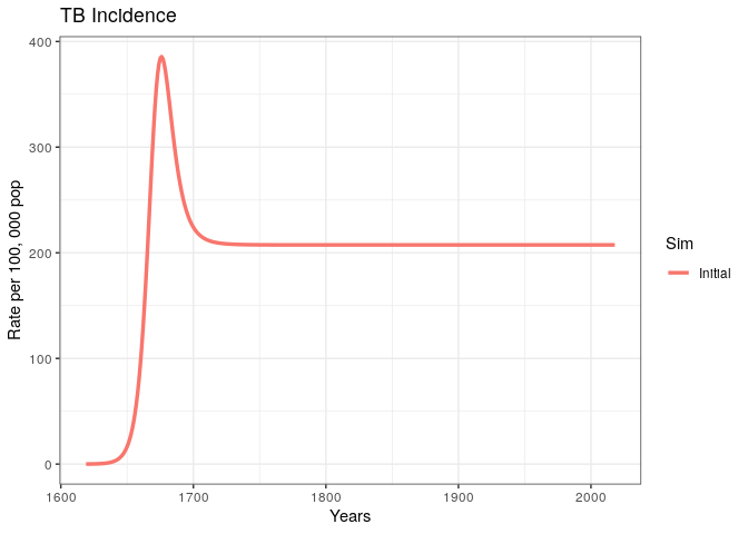

We have produced and incidence trajectory for a system that seems to be in endemic equilibrium.

4) What does it mean for an epidemic to achieve endemic equilibrium?

5) Using concepts from previous lectures, can you think of a simple mathematical expression for the endemic equilibrium in terms of the basic reproduction number ((R_0)) ?

We could estimate (R_0) for the given model by rearranging the terms in the previous equation; however, this would be incorrect because there are factors specific to the natural history of TB that interfere with the usual interpretation of the reproduction number.

6) Can you think of at least two factors specific to the natural history of TB that can complicate our interpretation of (R_0) and (R_t) ?

Part II: explore the case for TB elimination

Now that we have some understanding of TB dynamics, let’s explore the case of TB elimination using our model. To make the case more realistic, we will try to get our TB incidence trajectory to match the current estimates for a high TB burden country.

1) Explore WHO’s TB country profiles for the 30 countries with the highest TB burden ( here )

2) Select a country with an incidence trend that resembles the unchanged trend in our model. Then, take note of the TB incidence rate per 100,000 population (including HIV/TB).

3) In the code below, replace the missing variables for country incidence, country name, and beta parameter. Vary the value of beta until your incidence trajectory matches the data point in the plot (run the code as many times as necessary).

Copy and paste the code below

# :::::: FILL IN THE MISSING VALUES HERE 

Inc.country    <-  # TB incidence per 100,000 (including TB/HIV) 
country.name   <-  # e.g., "Sierra Leone"
params["beta"] <-  # Transmission rate per capita per year
# ::::::
  
  
# run the model
out0 <- get_intervention(xstart, params, NA, times, NA, NA, TB.Basic,
                         "Initial", NA) 

# plot
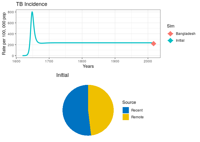
dot <- data.frame(Data = country.name, Years = 2017, incidence = Inc.country)

p1 <- out0$lines +
  geom_point(dot, mapping = aes(x = Years, y = incidence, col = Data), 
             size = 6, shape = 18) 

# Arrange plots in a grid
grid.arrange(p1, out0$pie)

Visually explore the model fit

4) Can you think of other ways in which the model parameters govern the overall size of the epidemic and the incidence rate at equilibrium?

Before we can start modelling interventions, we need a few more functions.

First, we need to create a wrapper function that allows us to scale-up our interventions smoothly over a period of time. Copy and execute the code below:

Copy and paste the code below

# Intervention scaling function
scale_up <- function(t, state, parameters, t.interv, parameters_old, fx) {
  
  scale <- min((t - t.interv[1])/(t.interv[2] - t.interv[1]), 1) 
  if (scale < 0) 
  {
    scale <- 0
  }
  
  pars_scaled <- parameters;
  
  pars_scaled <- parameters_old + scale * (parameters - parameters_old)
  
  return(fx(t, state, pars_scaled))
}

Let’s create some function handles to pass as arguments.

Copy and paste the code below

# Function handles

fx_basic <- TB.Basic
fx_scale <- function(t, state, parameters) scale_up(t, state, parameters, t.interv, params, fx_basic)

Now, let’s create a baseline incidence to use as a counterfactual in our exploration of TB elimination.

Copy and paste the code below

## Simulation 0
# Project at baseline
int_name    <- "Baseline"

# Initial conditions (starting in 2019)
sfin        <- tail(out0$out, 1)                             
params_base <- params
times_new   <- seq(t.intervention, t.intervention + 25, by = 1)
t.interv    <- c(times_new[2], times_new[2] + t.scale)

# Run model
data0 <- get_intervention(sfin, params_base, params_base, times_new, NA,
                          fx_scale, fx_basic, "Baseline", NA) 
# Plot
grid.arrange(data0$lines, data0$pie)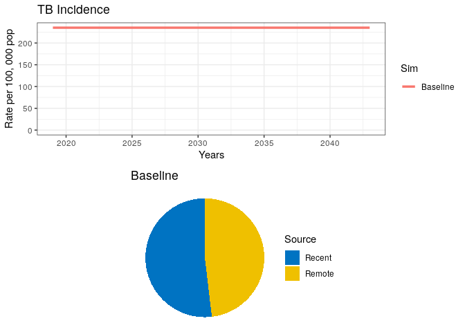

TB Treatment

We will start our exploration of interventions by simulating the roll-out of a successful TB treatment campaign. The simplest way is to alter the rate of spontaneous cure.

On the path to successful (curative) TB treatment, there are a number of events an individual may experience. For example:

1) Careseeking rate (cs): we define careseking as the time it takes for a symptomatic individual to seek medical care 2) Probability of diagnosis (pDx): the probability that once an individual has sought care, a diagnostic test will be performed 3) Probability of treatment (pTx): probability that once an individual has been diagnosed, treatment will be prescribed 4) Treatment duration (T.rtx): total duration of the treatment course (standard TB treatment is 6 months)

5) Can you list at least two other factors related to TB treatment success?

6) In the code below, assign values to the variables that reflect the components of TB treatment. Consider an average careseeking delay of 1 year, a probability of diagnosis of 95%, and treatment initiation of 95%.

7) Write the code for the term Tx (note that Tx is a rate that will add to the existing self-cure rate in your model). Run the code to see the results.

## Simulation 1
# An Intervention simulating introduction of treatment
int_name  <- "Treatment"

# Update parameter results data frame to append new results
params_1  <- params_base
data_stub <- data0$data

# :::: COMPLETE THE MISSING VALUES AND WRITE A TERM FOR RATE Tx

# Change parameters for intervention
T.cs  <-       # Time delay (yrs) between developing symptoms and seeking care
pDx   <-       # Probability of being diagnosed once care sought
pTx   <-       # probability of recieving correct Tx if diagnosed
T.rTx <- 0.5   # 6 months treatment duration
Tx    <-

# ::::
  
params_1["selfcure"] <- selfcure + Tx

data1 <- get_intervention(sfin, params_1, params_base, times_new, t.interv,
                          fx_scale, fx_basic, int_name, data_stub) 

p1 <- data1$lines +
  # EndTb
  geom_hline(yintercept = Inc.country*0.1, linetype = "dashed", color = "black", size = 1) +
  # Elimination
  geom_hline(yintercept = 0.1/1e5, linetype = "dashed", color = "red", size = 1)


grid.arrange(p1, data1$pie)

Your plot should look similar to the one below.

8) What can you say about the proportion of Recent vs. Remote ?

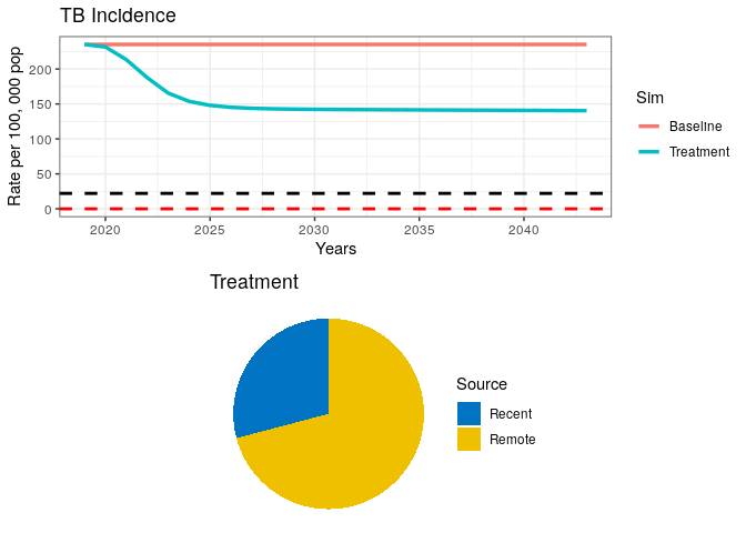
In the above plot, we have included dashed lines for WHO’s End TB goal (black) and a TB elimination threshold (red). This is so we can check how our model performs against these reference goals. WHO has defined the End TB goal as a 95% reduction in TB incidence by 2035. Elimination is defined as a threshold of <1 case per million population. The latter should be interpreted as the theoretical limit for eradication, while the End TB is meant to be an achievable goal, which, if achieved, should bring countries close to elimination.

Increase the Demand for TB Services

Now, let’s combine the treatment campaign with an intervention that makes TB services widely available in the community. This intervention should increase the current yield of TB prevalent cases screened by 75%.

9) What parameters in our previous simulation would you alter to simulate such an intervention? Modify the code below and run it.

(Note: remember that we want to combine interventions, i.e., the previous intervention should also be included here)

## Simulation 2
# An Intervention simulating demand generation
int_name  <- "Demand generation"

# Update parameter results data frame to append new results
params_2  <- params_1
data_stub <- data1$data

# ::::::: COMPLETE THE MISSING VALUES AND WRITE A NEW TERM FOR Tx

# Change parameters for intervention
T.cs  <-      # Time delay (yrs) between developing symptoms and seeking care
pDx   <-      # Probability of being diagnosed once care sought
pTx   <-      # probability of receiving correct Tx if diagnosed
T.rTx <-      # 6 months treatment duration

Tx    <-

# :::::::::::
  
  
params_2["selfcure"] <- selfcure + Tx

data2 <- get_intervention(sfin, params_2, params_base, times_new, t.interv,
                          fx_scale, fx_basic, int_name, data_stub) 

p1 <- data2$lines +
  # EndTb
  geom_hline(yintercept = Inc.country*0.1, linetype = "dashed", color = "black", size = 1) +
  # Elimination
  geom_hline(yintercept = 0.1/1e5, linetype = "dashed", color = "red", size = 1)


grid.arrange(p1, data2$pie )

Our plot should look like this:

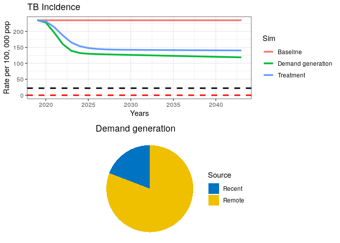
We can see from our remote/recent pie chart that even after a strong combined campaign to reduce TB burden, some transmission remains.

TB Transmission Control

Let’s imagine a hypothetical scenario where transmission is completely stopped. This is unrealistic, but for the sake of testing our elimination case, let’s imagine we can stop transmission with a fully curative intervention in every single prevalent case.

10) Run the code below.

Copy and paste the code below

## Simulation 3
int_name  <- "Transmission stop"

# Update parameter results data frame to append new results
params_3  <- params_2
data_stub <- data2$data

# An Intervention simulating transmission reduction

params_3["beta"] <- 0


data3 <- get_intervention(sfin, params_3, params_base, times_new, t.interv,
                          fx_scale, fx_basic, int_name, data_stub) 

p1 <- data3$lines +
  # EndTb
  geom_hline(yintercept = Inc.country*0.1, linetype = "dashed", color = "black", size = 1) +
  # Elimination
  geom_hline(yintercept = 0.1/1e5, linetype = "dashed", color = "red", size = 1)


grid.arrange(p1, data3$pie)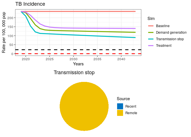

A fully curative intervention appears insufficient to drive the TB epidemic to elimination.

11) If transmission has stopped (as seen in the pie chart), where is the remaining incidence coming from?

12) Where should we intervene to finally drive the TB epidemic down?

LTBI Treatment

Let’s introduce a prevention campaign that treats 100% of all latent TB infections (LTBI) and reduces progression to active TB in 99% of them.

13) Run the code below

(Note that the black dashed line below represents the End TB goal and the red dashed line is the elimination threshold)

Copy and paste the code below

## Simulation 4
# An Intervention simulating LTBI treatment
int_name  <- "Prevention"

# Update parameter results data frame to append new results
params_4  <- params_3
data_stub <- data3$data

params_4["break_in"] <- 0.01 * (1/T.lfx)

data4 <- get_intervention(sfin, params_4, params_base, times_new,
                          t.interv, fx_scale, fx_basic, int_name, data_stub) 

p1 <- data4$lines +
  # EndTb
  geom_hline(yintercept = Inc.country*0.1, linetype = "dashed", color = "black", size = 1) +
  # Elimination
  geom_hline(yintercept = 0.1/1e5, linetype = "dashed", color = "red", size = 1)


grid.arrange(p1, data4$pie)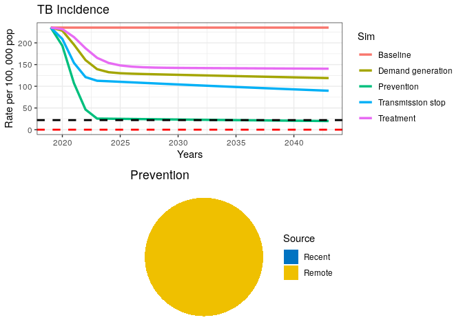

This final intervention scenario reaches the goal for End TB just before 2035 but is still far from elimination.

We have coded and run a simple TB model for exploring the case of TB elimination and WHO’s End TB goal. Even though we did not perform rigorous analyses on this subject, our simple exercise suggests that a combination of curative and preventive measures will be required to achieve End TB goals in a high burden setting.

Finally, take a few minutes to think about how the following added complexities to the model could affect our estimations:

1) Age structure

2) Risk groups (e.g. HIV/AIDS, slum dwellers, diabetes, malnourishment)

3) MDR-TB