An introduction to R and RStudio
Introduction
This tutorial is part of the pre-course materials of a “Short Course on Outbreak Analysis and Modelling for Public Health.” The aim is to introduce students to the very basic concepts of R and R Studio, in order to get some baseline knowledge in R and R programming.
Installing R and R Studio
R is a free software environment and RStudio is a free and open-source environment for working in R. Both R and Studio should be installed separately.
R can be installed from the R Project for Statistical computing website: https://r-project.org/
RStudio can be installed from its website. The free version is
sufficient to conduct routine epidemiological analyses
https://www.rstudio.com/products/rstudio/download/
Once both are installed, we work from RStudio.
For a very detailed explanation on how to install R and R Studio, please visit the video made by Thibaut Jombart from RECON https://www.youtube.com/watch?v=LbezGA_Yle8
Project setup
One of the great advantages of using RStudio is the possibility of using
R Projects (indicated by an .Rproj file) to organise the work space,
history, and source documents.
To create this, do the following steps:
- Open RStudio and on the top right corner find New Project
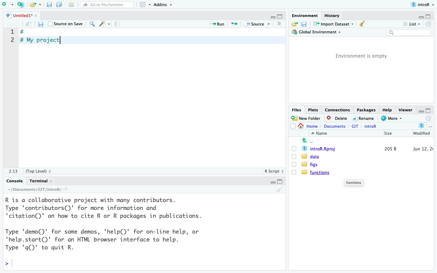
- Create a new RStudio project in a new directory that you can call “introR”
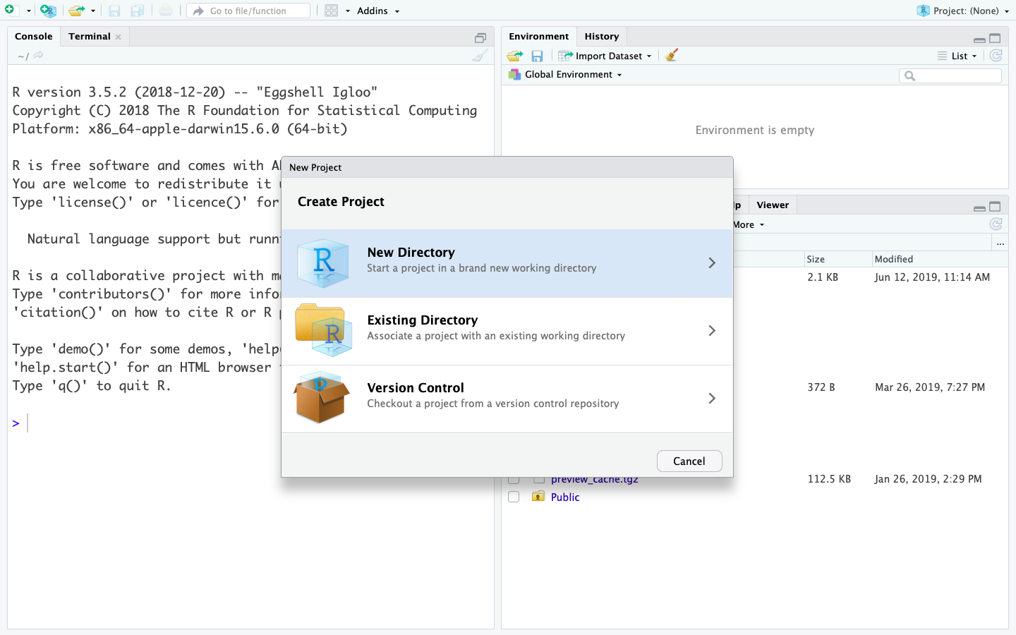
- Create the sub folders you need for organising your work (i.e. data, scripts, figs)
In the end, your project should look something like this image
Structures in R
According to Hadley Wickham, in his Advanced R book [http://adv-r.had.co.nz/], there are two types of structures in R:
- Homogeneous: atomic vectors (1d), matrices (2d), and arrays (nd)
- Heterogeneous: data frames and lists
Atomic vectors
These are the most basic structures in R and have only one dimension (1d):
- Double (numeric)
- Logic
- Character
- Integer
vector_double <- c(1, 2, 3, 4)
vector_logic <- c(TRUE, FALSE, FALSE, TRUE)
vector_character <- c("A", "B", "C", "D")
vector_integer <- c(1L, 2L, 3L, 4L)To evaluate which type of vector we have, we can use two commands
typeof
typeof(vector_double)
## [1] "double"
typeof(vector_logic)
## [1] "logical"
typeof(vector_character)
## [1] "character"
typeof(vector_integer)
## [1] "integer"Matrices
Matrices are structures a bit more complex than vectors, with two main characteristics:
- A matrix is composed of only one type of vector
- A matrix has two dimensions
A command to build a matrix uses three arguments:
datacorresponds to the list of vectors we want to use in the matrixnrowthe number of rows where the data is going to be split (first dimension)ncolthe number of columns where the data is going to be split (second dimension)
By default the matrix is filled by column, unless we specify otherwise
using byrow = TRUE
matrix_of_doub <- matrix(data = vector_double, nrow = 2, ncol = 2)
matrix_of_doub
## [,1] [,2]
## [1,] 1 3
## [2,] 2 4
dim(matrix_of_doub)
## [1] 2 2Make and test other types of matrices
matrix_of_log <- matrix(data = vector_logic, nrow = 4, ncol = 3)
matrix_of_log
matrix_of_char <- matrix(data = vector_character, nrow = 4, ncol = 4)
matrix_of_char
matrix_of_int <- matrix(data = vector_integer, nrow = 4, ncol = 5)
matrix_of_intArrays
Array is a special type of matrix, where there is more than two dimensions (n dimensions).
An array of two dimensions is a matrix
To create an array we need three arguments: data and dim.
In turn, the dim argument of an array is composed of three arguments
being: 1) number of rows, 2) number of columns and 3) number of
dimensions.
vector_example <-1:18
array_example <- array(data = vector_example, dim = c(2, 3, 3))
dim(array_example)
## [1] 2 3 3
array_example
## , , 1
##
## [,1] [,2] [,3]
## [1,] 1 3 5
## [2,] 2 4 6
##
## , , 2
##
## [,1] [,2] [,3]
## [1,] 7 9 11
## [2,] 8 10 12
##
## , , 3
##
## [,1] [,2] [,3]
## [1,] 13 15 17
## [2,] 14 16 18Data frames
A data.frame is a heterogeneous and bi dimensional structure, similar
but not exactly equal to a matrix. Unlike a matrix, various types of
vectors can be part of a single data frame.
The arguments for the data.frame command are simply the columns in the
data frame. Each column should have the same number of rows to be able
to fit into a data frame.
Data frames do not allow vectors with different lengths. When the length of the vector is smaller than the length of the data frame, the data frame coerces the vector to its length.
data_example <- data.frame(vector_character, vector_double, vector_logic, vector_integer)To access the general structure of a data frame we use the command str
str(data_example)
## 'data.frame': 4 obs. of 4 variables:
## $ vector_character: chr "A" "B" "C" "D"
## $ vector_double : num 1 2 3 4
## $ vector_logic : logi TRUE FALSE FALSE TRUE
## $ vector_integer : int 1 2 3 4To access the different components of the data frame we use this syntax
[,] where the first dimension corresponds to rows and the second
dimension to columns.
data_example[1, 2]
## [1] 1Lists
A list is the most complex structure in base R. A list can be composed
of any type of objects of any dimension.
list_example <- list(vector_character,
matrix_of_doub,
data_example)To access the different components of a list, we use the syntax []
where the argument is simply the order within the list.
list_example[1]
## [[1]]
## [1] "A" "B" "C" "D"Functions
A function is one of the structures that makes R a very powerful platform for programming.
There are various types of functions
- Primitive or base functions: these are the default functions in
R under the base package. For instance, these can include basic
arithmetic operations, but also more complex operations such as
extraction of median values
medianorsummaryof a variable. - Functions from packages : these are functions created within a
package. For example the function
glmin the stats package. - User-built functions: these are functions that any user creates for a customized routine. These functions could become part of a package.
The basic components of a function are:
- name: this is the name that we give to our function (for example:
myfun) - formals or arguments: these are the series of elements that control how to call the function.
- body: this is the series of operations or modifications to the arguments.
- output: this is the results after modifying the arguments. If this
output corresponds to a series of data, we can extract it using the
command
return. - function internal environment: means the specific rules and objects within a function. Those rules and objects will not work outside the function.
User-built function (example 1)
Let’s build a function that calculates our Body Mass Index (BMI)
# The name (myfun)
myfun <- function(weight,
height) # The arguments (weight and height)
{
# The body
BMI <- weight/(height^2)
return(BMI) # Retun specification for the output
}
formals(myfun)
## $weight
##
##
## $height
body(myfun)
## {
## BMI <- weight/(height^2)
## return(BMI)
## }
environment(myfun)
## <environment: R_GlobalEnv>
myfun(weight = 88, height = 1.78)
## [1] 27.77427User-built function (example 2)
Let’s build a function that has default values. This way, we don’t need to specify some of the arguments as they can be set by default.
# The name (myfun2)
myfun2 <- function(weight,
height,
units = 'kg/m2') # The arguments (weight and height)
{
# The body
BMI <- weight/(height^2)
output <- paste(round(BMI, 1), units)
return(output) # Retun specification for the output
}
myfun2(weight = 88, height = 1.78)
## [1] "27.8 kg/m2"
myfun2(weight = 8800, height = 178, units = 'g/cm2')
## [1] "0.3 g/cm2"R packages
As described by Hadley Wickham in his book R packages, a package is the fundamental unit of reproducible R code. A package should include at least:
- Reusable R functions
- Documentation
- Sample data
Any R user can build a package that can then be used or modified by others as they are open-source.
The R packages are available on the Comprehensive R Archive Network (CRAN) https://cran.r-project.org
Here are the basic commands to use packages:
- Install a package with the command
install.packages("package-name") - Use them in R with
library("package-name")
Let’s install one of the packages from RECON.
install.packages('incidence')
library(incidence)Library is a directory containing installed packages. We can use
lapply(.libPaths(), dir) to check which packages are active currently
in our R session.
An important part of a package is the documentation. This is stored in
the vignettes. To access the basic documentation on a package we can
use browseVignettes("incidence")
Scoping and Environments
A new environment is created when we create a function. This is important! When we call a function, R first looks for the elements within that function; if the elements do not exist within that function, then R looks for them in the global environment.
- Example of a function in which objects are only avalible in the global environment
mynewfun <- function() {
z = x + y
return(z)
}
x = 1
y = 3
mynewfun()
## [1] 4- Example of a function in which objects are defined partially in the local environment and partially in the global envoronment
mynewfun <- function(xx) {
zz = xx + yy
return(zz)
}
yy = 4
mynewfun(xx = 4)
## [1] 8This characteristic of R is very important when running any analysis or routine. It is always recommended to NOT use elements within a function that are only available in the global environment.
Working with probability distributions
All distributions in R can be explored by the use of functions that allow us to get different forms of a distribution. Fortunately, all distributions work in the same way, so if you learn to work with one, you will have the general idea of how to work with the others
For example, for a normal distribution we use ?dnorm to explore the
arguments in this function
dnorm= density function with default arguments(x, mean = 0, sd = 1, log = FALSE)pnormgives the distribution functionqnormgives the quantile functionrnormgenerates random deviates
Many distributions are part of the stats package that comes by default
with R such as the uniform, poisson, and binomial, among others.
For other less frequently used distributions, sometimes you may need to
install other packages. For a non-exhaustive list of the most used
distrubutions and their arguments, see the table below:
| name | probability | quantile | distribution | random |
|---|---|---|---|---|
| Beta | pbeta() |
qbeta() |
dbeta() |
rbeta() |
| Binomial | pbinom() |
qbinom() |
dbinom() |
rbinom() |
| Cauchy | pcauchy() |
qcauchy() |
dcauchy() |
rcauchy() |
| Chi-Square | pchisq() |
qchisq() |
dchisq() |
rchisq() |
| Exponential | pexp() |
qexp() |
dexp() |
rexp() |
| Gamma | pgamma() |
qgamma() |
dgamma() |
rgamma() |
| Logistic | plogis() |
qlogis() |
dlogis() |
rlogis() |
| Log Normal | plnorm() |
qlnorm() |
dlnorm() |
rlnorm() |
| Negative Binomial | pnbinom() |
qnbinom() |
dnbinom() |
rnbinom() |
| Normal | pnorm() |
qnorm() |
dnorm() |
rnorm() |
| Poisson | ppois() |
qpois() |
dpois() |
rpois() |
| Student’s t | pt() |
qt() |
dt() |
rt() |
| Uniform | punif() |
qunif() |
dunif() |
runif() |
| Weibull | pweibull() |
qweibull() |
dweibull() |
rweibull() |
Create and open data sets
R allows users not only to open but also to create data sets. There are three sources of data sets:
- Data set imported as such (from
.xlsx,.csv,.stata, or.RDSformats, among many others) - Data set that is part of a R package
- Data set created in our R session
Tidyverse
In order to better manage data sets, we recommend installing and using
the tidyverse package, which automatically uploads several packages
(dplyr, tidyr, tibble, readr, purr, among others) that are useful for
data wrangling.
library(tidyverse)Let’s open and explore a data set imported from Excel
This is the data set from our RECON practical on early outbreak analysis: - PHM-EVD-linelist-2017-11-25.xlsx:
Let’s save this data set in the same directory in which we are currently working.
To import data sets from Excel, we can use the library readxl, which
is linked to tidyverse. However, we still need to load the readxl
library, as it is not a core tidyverse package.
library(readxl)
library(here)
dat <- read_excel(here("data/PHM-EVD-linelist-2017-11-25.xlsx"))Next, we will take a look at some of the most commonly used functions
from tidyverse.
We will be using the pipe function %>% often. This is key to using
tidyverse and makes programming easier. The pipe function allows the
user to emphasize a sequence of actions on an object.
From the package dyplr, the most common functions are:
glimpse: used to rapidly explore a data setarrange: arranges the data set by the value of a particular variable if numeric, or by alphabetic order if it is a character.mutate: generates a new variablerename: changes a variable’s namesummarise: reduces the dimensions of a data set
glimpse(dat)
## Rows: 50
## Columns: 4
## $ case_id <chr> "39e9dc", "664549", "b4d8aa", "51883d", "947e40", "9aa197", "e~
## $ onset <dttm> 2017-10-10, 2017-10-16, 2017-10-17, 2017-10-18, 2017-10-20, 2~
## $ sex <chr> "female", "male", "male", "male", "female", "female", "female"~
## $ age <dbl> 62, 28, 54, 57, 23, 66, 13, 10, 34, 11, 23, 23, 9, 68, 37, 13,~
dat %>% arrange(age)
## # A tibble: 50 x 4
## case_id onset sex age
## <chr> <dttm> <chr> <dbl>
## 1 ac8d9d 2017-11-23 00:00:00 female 5
## 2 8c5776 2017-11-02 00:00:00 female 7
## 3 426b6d 2017-11-08 00:00:00 female 7
## 4 93a3ba 2017-11-10 00:00:00 male 7
## 5 5eb2b0 2017-11-13 00:00:00 female 7
## 6 1efd54 2017-11-04 00:00:00 male 8
## 7 e37897 2017-10-28 00:00:00 female 9
## 8 59e66c 2017-11-16 00:00:00 male 9
## 9 af0ac0 2017-10-21 00:00:00 male 10
## 10 778316 2017-11-04 00:00:00 female 10
## # ... with 40 more rows
dat %>% mutate(fecha_inicio_sintomas = onset)
## # A tibble: 50 x 5
## case_id onset sex age fecha_inicio_sintomas
## <chr> <dttm> <chr> <dbl> <dttm>
## 1 39e9dc 2017-10-10 00:00:00 female 62 2017-10-10 00:00:00
## 2 664549 2017-10-16 00:00:00 male 28 2017-10-16 00:00:00
## 3 b4d8aa 2017-10-17 00:00:00 male 54 2017-10-17 00:00:00
## 4 51883d 2017-10-18 00:00:00 male 57 2017-10-18 00:00:00
## 5 947e40 2017-10-20 00:00:00 female 23 2017-10-20 00:00:00
## 6 9aa197 2017-10-20 00:00:00 female 66 2017-10-20 00:00:00
## 7 e4b0a2 2017-10-21 00:00:00 female 13 2017-10-21 00:00:00
## 8 af0ac0 2017-10-21 00:00:00 male 10 2017-10-21 00:00:00
## 9 185911 2017-10-21 00:00:00 female 34 2017-10-21 00:00:00
## 10 601d2e 2017-10-22 00:00:00 male 11 2017-10-22 00:00:00
## # ... with 40 more rows
dat %>% rename(edad = age)
## # A tibble: 50 x 4
## case_id onset sex edad
## <chr> <dttm> <chr> <dbl>
## 1 39e9dc 2017-10-10 00:00:00 female 62
## 2 664549 2017-10-16 00:00:00 male 28
## 3 b4d8aa 2017-10-17 00:00:00 male 54
## 4 51883d 2017-10-18 00:00:00 male 57
## 5 947e40 2017-10-20 00:00:00 female 23
## 6 9aa197 2017-10-20 00:00:00 female 66
## 7 e4b0a2 2017-10-21 00:00:00 female 13
## 8 af0ac0 2017-10-21 00:00:00 male 10
## 9 185911 2017-10-21 00:00:00 female 34
## 10 601d2e 2017-10-22 00:00:00 male 11
## # ... with 40 more rows
glimpse(dat)
## Rows: 50
## Columns: 4
## $ case_id <chr> "39e9dc", "664549", "b4d8aa", "51883d", "947e40", "9aa197", "e~
## $ onset <dttm> 2017-10-10, 2017-10-16, 2017-10-17, 2017-10-18, 2017-10-20, 2~
## $ sex <chr> "female", "male", "male", "male", "female", "female", "female"~
## $ age <dbl> 62, 28, 54, 57, 23, 66, 13, 10, 34, 11, 23, 23, 9, 68, 37, 13,~
dat %>% group_by(sex) %>% summarise(number = n())
## # A tibble: 2 x 2
## sex number
## <chr> <int>
## 1 female 26
## 2 male 24
dat %>% filter(age >14)
## # A tibble: 34 x 4
## case_id onset sex age
## <chr> <dttm> <chr> <dbl>
## 1 39e9dc 2017-10-10 00:00:00 female 62
## 2 664549 2017-10-16 00:00:00 male 28
## 3 b4d8aa 2017-10-17 00:00:00 male 54
## 4 51883d 2017-10-18 00:00:00 male 57
## 5 947e40 2017-10-20 00:00:00 female 23
## 6 9aa197 2017-10-20 00:00:00 female 66
## 7 185911 2017-10-21 00:00:00 female 34
## 8 605322 2017-10-22 00:00:00 female 23
## 9 e399b1 2017-10-23 00:00:00 female 23
## 10 f658bc 2017-10-28 00:00:00 male 68
## # ... with 24 more rows
select(dat, starts_with("date"))
## # A tibble: 50 x 0
select(dat, ends_with("loc"))
## # A tibble: 50 x 0
slice(dat, 10:15)
## # A tibble: 6 x 4
## case_id onset sex age
## <chr> <dttm> <chr> <dbl>
## 1 601d2e 2017-10-22 00:00:00 male 11
## 2 605322 2017-10-22 00:00:00 female 23
## 3 e399b1 2017-10-23 00:00:00 female 23
## 4 e37897 2017-10-28 00:00:00 female 9
## 5 f658bc 2017-10-28 00:00:00 male 68
## 6 a8e9d8 2017-10-29 00:00:00 female 37
dat[10:15, ]
## # A tibble: 6 x 4
## case_id onset sex age
## <chr> <dttm> <chr> <dbl>
## 1 601d2e 2017-10-22 00:00:00 male 11
## 2 605322 2017-10-22 00:00:00 female 23
## 3 e399b1 2017-10-23 00:00:00 female 23
## 4 e37897 2017-10-28 00:00:00 female 9
## 5 f658bc 2017-10-28 00:00:00 male 68
## 6 a8e9d8 2017-10-29 00:00:00 female 37
filter(dat, sex == "female", age <= 30)
## # A tibble: 19 x 4
## case_id onset sex age
## <chr> <dttm> <chr> <dbl>
## 1 947e40 2017-10-20 00:00:00 female 23
## 2 e4b0a2 2017-10-21 00:00:00 female 13
## 3 605322 2017-10-22 00:00:00 female 23
## 4 e399b1 2017-10-23 00:00:00 female 23
## 5 e37897 2017-10-28 00:00:00 female 9
## 6 8c5776 2017-11-02 00:00:00 female 7
## 7 88526e 2017-11-03 00:00:00 female 20
## 8 778316 2017-11-04 00:00:00 female 10
## 9 525dfa 2017-11-06 00:00:00 female 10
## 10 b5ad13 2017-11-07 00:00:00 female 21
## 11 8bed66 2017-11-08 00:00:00 female 29
## 12 426b6d 2017-11-08 00:00:00 female 7
## 13 c2a389 2017-11-10 00:00:00 female 26
## 14 5eb2b0 2017-11-13 00:00:00 female 7
## 15 b7faf4 2017-11-16 00:00:00 female 10
## 16 944ba3 2017-11-19 00:00:00 female 30
## 17 95fc1d 2017-11-19 00:00:00 female 15
## 18 5c5c05 2017-11-20 00:00:00 female 21
## 19 ac8d9d 2017-11-23 00:00:00 female 5Let’s open and explore a data set that is part of a package
# install.packages("outbreaks")
library(outbreaks)
## Warning: package 'outbreaks' was built under R version 4.0.4
measles_dat <- outbreaks::measles_hagelloch_1861
class(measles_dat)
## [1] "data.frame"
head(measles_dat)
## case_ID infector date_of_prodrome date_of_rash date_of_death age gender
## 1 1 45 1861-11-21 1861-11-25 <NA> 7 f
## 2 2 45 1861-11-23 1861-11-27 <NA> 6 f
## 3 3 172 1861-11-28 1861-12-02 <NA> 4 f
## 4 4 180 1861-11-27 1861-11-28 <NA> 13 m
## 5 5 45 1861-11-22 1861-11-27 <NA> 8 f
## 6 6 180 1861-11-26 1861-11-29 <NA> 12 m
## family_ID class complications x_loc y_loc
## 1 41 1 yes 142.5 100.0
## 2 41 1 yes 142.5 100.0
## 3 41 0 yes 142.5 100.0
## 4 61 2 yes 165.0 102.5
## 5 42 1 yes 145.0 120.0
## 6 42 2 yes 145.0 120.0
tail(measles_dat)
## case_ID infector date_of_prodrome date_of_rash date_of_death age gender
## 183 183 184 1861-11-11 1861-11-15 <NA> 4 m
## 184 184 NA 1861-10-30 1861-11-06 <NA> 13 <NA>
## 185 185 82 1861-12-03 1861-12-07 <NA> 3 m
## 186 186 45 1861-11-22 1861-11-26 <NA> 6 <NA>
## 187 187 82 1861-12-07 1861-12-11 <NA> 0 m
## 188 188 175 1861-11-23 1861-11-27 <NA> 1 <NA>
## family_ID class complications x_loc y_loc
## 183 4 0 yes 182.5 200.0
## 184 51 2 yes 182.5 200.0
## 185 21 0 yes 205.0 182.5
## 186 57 0 yes 212.5 90.0
## 187 21 0 yes 205.0 182.5
## 188 57 0 yes 212.5 90.0From the package tidyr, the most common functions are:
gather: makes wide data longerspread: makes long data wider
Example:
malaria <- tibble(
name = letters[1:10],
age = round(rnorm(10, 30, 10), 0),
gender = rep(c('f', 'm'), 5),
infection = rep(c('falciparum', 'vivax', 'vivax', 'vivax', 'vivax'), 2)
)
glimpse(malaria)
## Rows: 10
## Columns: 4
## $ name <chr> "a", "b", "c", "d", "e", "f", "g", "h", "i", "j"
## $ age <dbl> 29, 41, 39, 22, 33, 32, 48, 27, 37, 24
## $ gender <chr> "f", "m", "f", "m", "f", "m", "f", "m", "f", "m"
## $ infection <chr> "falciparum", "vivax", "vivax", "vivax", "vivax", "falciparu~
malaria %>% spread(key = 'infection', gender)
## # A tibble: 10 x 4
## name age falciparum vivax
## <chr> <dbl> <chr> <chr>
## 1 a 29 f NA
## 2 b 41 NA m
## 3 c 39 NA f
## 4 d 22 NA m
## 5 e 33 NA f
## 6 f 32 m NA
## 7 g 48 NA f
## 8 h 27 NA m
## 9 i 37 NA f
## 10 j 24 NA mggplot2
ggplot is an implementation of the concept of grammar of graphics
that has been implemented in R by Hadley Wickham. He explains in his
ggplot2 book that “the grammar is a mapping from data to aesthetic
attributes (colour, shape, size) of geometric objects (points, lines,
bars).”
The main components of a ggplot2 plot are:
- data frame
- aesthesic mappings this refers to the indications on how the data should be mapped (x, y) to colour, size, etc
- geoms refers to geometric objects such as points, lines, shapes
- facets for conditional plots
- coodinate system
Basic functions in ggplot
ggplot() is the core function in ggplot2. The basic argument of the
function is the data frame we want to plot (data). ggplot(data) then
can be associated using the symbol + to other types of functions, such
as the geoms that will draw a particular type of shape. Some of the
most commonly used are:
geom_point(): for pointsgeom_line(): for linesgeom_bar(): for bar chartsgeom_histogram(): for histograms
All of these commands will use the same syntax for the aesthetics
(x, y, colour, fill, shape).
GGplot example with the measles data set
Let’s use the measles data set from the outbreaks package that we
imported above. In this case, we want to make a graph that displays the
time-series of cases by week coloured by gender. We have to define that:
x= timey= aggregated number of cases by week and gendercolour= gender
An important thing to be of aware is that for a single instruction, ggplot will only use variables that belong to the same data set. So, we need to have the three variables (x, y, and colour) in the same data frame (with the same length).
head(measles_dat, 5)
## case_ID infector date_of_prodrome date_of_rash date_of_death age gender
## 1 1 45 1861-11-21 1861-11-25 <NA> 7 f
## 2 2 45 1861-11-23 1861-11-27 <NA> 6 f
## 3 3 172 1861-11-28 1861-12-02 <NA> 4 f
## 4 4 180 1861-11-27 1861-11-28 <NA> 13 m
## 5 5 45 1861-11-22 1861-11-27 <NA> 8 f
## family_ID class complications x_loc y_loc
## 1 41 1 yes 142.5 100.0
## 2 41 1 yes 142.5 100.0
## 3 41 0 yes 142.5 100.0
## 4 61 2 yes 165.0 102.5
## 5 42 1 yes 145.0 120.0From the above command, we notice that the measles data set does not
currently contain one of the three variables, the y variable
(aggregated number of cases per week, by gender). This means we first
need to reformat the data frame so that it contains the three variables
we want to plot.
To reformat the data frame, we can use various functions explained above
from the dplyr package.
measles_grouped <- measles_dat %>%
filter(!is.na(gender)) %>%
group_by(date_of_rash, gender) %>%
summarise(cases = n())
## `summarise()` has grouped output by 'date_of_rash'. You can override using the `.groups` argument.
head(measles_grouped, 5)
## # A tibble: 5 x 3
## # Groups: date_of_rash [4]
## date_of_rash gender cases
## <date> <fct> <int>
## 1 1861-11-03 m 1
## 2 1861-11-08 f 1
## 3 1861-11-11 f 1
## 4 1861-11-11 m 1
## 5 1861-11-13 m 1Once the data frame is ready, plotting is easy:
ggplot(data = measles_grouped) +
geom_line(aes(x = date_of_rash, y = cases, colour = gender))
By default, ggplot makes several decisions for us, such as the colours used, the size of the lines, the font size, etc. Sometimes we may want to change them to improve the visualisation.
Here is an alternative way of presenting the same data. Modify some of the lines, and see how the plot changes.
p <- ggplot(data = measles_grouped,
aes(x = date_of_rash, y = cases, fill = gender)) +
geom_bar(stat = 'identity', colour = 'black', alpha = 0.5) +
facet_wrap(~ gender, nrow = 2) +
xlab('Date of onset') +
ylab('measles cases') +
ggtitle('Measles Cases in Hagelloch (Germany) in 1861') +
theme(strip.background = element_blank(),
strip.text.x = element_blank()) +
theme(legend.position = c(0.9, 0.2)) +
scale_fill_manual(values =c('purple', 'green'))
p
Finally, ggplot has a useful feature that allows users to add layers on top of existing ggplot objects. For instance, if we decide to change the title and colour of the gender variable after we finished the plot, we do not have to make the plot again. We simply add a command to overwrite the previous plot.
p +
ggtitle('another title') +
scale_fill_manual(values =c('blue', 'lightblue'))
## Scale for 'fill' is already present. Adding another scale for 'fill', which
## will replace the existing scale.
Further learning
To apply these basic concepts to a particular case, I recommend doing the practical “An outbreak of gastroenteritis in Stegen, Germany” from the RECON learn website https://www.reconlearn.org/post/stegen.html
Recommended readings
Much of the content for this basic R tutorial came from well-known books by Hadley Wickham which are mostly available online.
- R for Data Science https://r4ds.had.co.nz/index.html
- Advanced R http://adv-r.had.co.nz/
- R packages http://r-pkgs.had.co.nz/
Contributors
- Zulma M. Cucunuba: initial version
- Zhian N. Kamvar: minor edits
- Kelly A. Charniga: minor edits
Contributions are welcome via pull requests.
Legal stuff
License: CC-BY Copyright: Zulma M. Cucunuba, 2019
Contributions are welcome via pull requests. The source file of this document can be found here.
You are free:
- to Share - to copy, distribute and transmit the work
- to Remix - to adapt the work Under the following conditions:
- Attribution - You must attribute the work in the manner specified by the author or licensor (but not in any way that suggests that they endorse you or your use of the work). The best way to do this is to keep as it is the list of contributors: sources, authors and reviewers.
- Share Alike - If you alter, transform, or build upon this work, you may distribute the resulting work only under the same or similar license to this one. Your changes must be documented. Under that condition, you are allowed to add your name to the list of contributors.
- You cannot sell this work alone but you can use it as part of a teaching. With the understanding that:
- Waiver - Any of the above conditions can be waived if you get permission from the copyright holder.
- Public Domain - Where the work or any of its elements is in the public domain under applicable law, that status is in no way affected by the license.
- Other Rights - In no way are any of the following rights affected by the license:
- Your fair dealing or fair use rights, or other applicable copyright exceptions and limitations;
- The author’s moral rights;
- Rights other persons may have either in the work itself or in how the work is used, such as publicity or privacy rights.
- Notice - For any reuse or distribution, you must make clear to others the license terms of this work by keeping together this work and the current license. This licence is based on http://creativecommons.org/licenses/by-sa/3.0/